
Gold rose 130-fold. Against M2, the gain was 1.66-fold.
Gold, U.S. equities and Bitcoin returns look different when money-supply growth becomes the denominator.

Gold’s dollar price increased approximately 130 times between a 1959 reference price and August 2026. Over the corresponding comparison window, U.S. M2 increased about 78 times. Divide one growth factor by the other and gold’s gain becomes 1.66 times, equivalent to roughly 0.76% annually relative to M2.
The S&P 500, including reinvested dividends, delivered approximately 10.57% nominal annualized growth over the same window. Dividing its growth by M2’s leaves 3.57% annually. Those results come from the source values and conventions documented below—not from subtracting rounded headline rates. Data and calculations
This is an alternative benchmark, not a replacement definition of inflation. The Consumer Price Index measures changes in prices paid by consumers for goods and services. M2 measures a stock of broad money. A return adjusted for one answers a different question from a return adjusted for the other. BLS, Federal Reserve
What happens when the denominator compounds?
Nominal returns describe how many more dollars an investment is worth. M2-adjusted returns describe whether that investment’s value grew faster than the selected money aggregate.
Let an asset’s value rise from A₀ to A₁ over n years, while M2 rises from M₀ to M₁. The relevant wealth ratio is:
M2-relative wealth = (A₁ / A₀) ÷ (M₁ / M₀)
Annualizing that ratio gives:
Adjusted CAGR = (1 + nominal CAGR) ÷ (1 + M2 CAGR) − 1
CAGR is the constant annual rate that connects two endpoints. Actual annual returns can vary widely along the way.
Consider an illustrative asset growing 7% annually while M2 grows 6.7%. Its adjusted CAGR is 1.07 / 1.067 − 1 = 0.281%, rather than 0.3%. Over 30 years, the asset becomes 7.61 times its starting value, while M2 becomes 7.00 times its starting value. The ratio rises only 1.09 times. Reproducible calculation
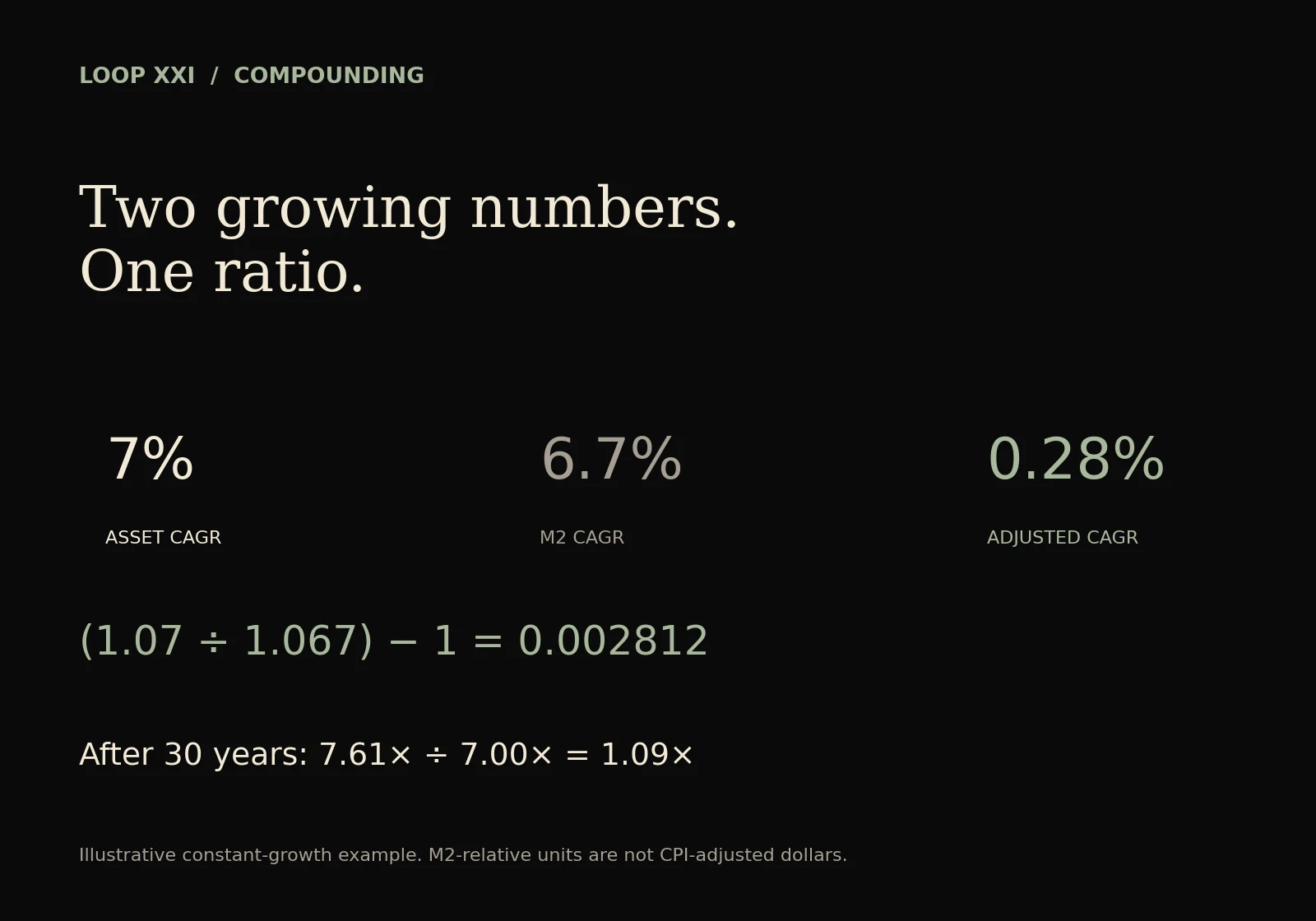
Compounding applies to both quantities.
Subtracting the two CAGRs is an approximation. Algebraically, the exact adjusted rate is (asset CAGR − M2 CAGR) / (1 + M2 CAGR). Simple subtraction omits that denominator and overstates a positive adjusted return when M2 growth is positive. It is especially unsuitable for comparing very high asset returns.
These ratios should not be called literal consumer purchasing power. M2 does not measure the price of food, housing or any other consumption basket. “Purchasing power relative to M2” is shorthand for a monetary-relative wealth index, not a quantity of goods an investor can buy.
The historical denominator
The Federal Reserve’s monthly, seasonally adjusted M2 series begins in January 1959 at $286.6 billion. Its latest observation, August 2026, is $23,342.8 billion, released September 22. That is 81.45-fold growth, or 6.73% annualized across 811 monthly intervals. FRED M2SL, downloaded observations

Monthly observations; logarithmic scale. Equal vertical distances represent equal proportional changes.
M2 is also distinct from the monetary base, which the Federal Reserve reports separately. The benchmark here is M2 throughout.
For the asset comparison, the starting convention is December 31, 1959, enabling use of a documented annual equity return series. December 1959 M2 was $297.8 billion. From that month to August 2026, its annualized growth is 6.76%. The 6.73% full-history rate and 6.76% matched-comparison rate therefore have different starting observations; they are not interchangeable.
Gold and equities: the long comparison
| Asset or benchmark | Reference period | Nominal CAGR | M2-adjusted CAGR |
|---|---|---|---|
| Gold, with 1959 price proxy | End-1959–August 2026 | 7.57% | 0.76% |
| S&P 500, dividends reinvested | End-1959–August 2026 | 10.57% | 3.57% |
| U.S. M2 | December 1959–August 2026 | 6.76% | 0.00% |
Calculations use unrounded inputs. These are gross benchmark returns before fees, taxes and implementation costs.
Gold begins at $35.10 per troy ounce, the 1959 annual average in NYU professor Aswath Damodaran’s historical dataset. It ends at the World Gold Council’s reported $4,563 for August 31, 2026. The starting price is an explicit proxy, not an independently observed December 31 close. Using the historical $35 official parity instead changes the adjusted CAGR only to about 0.77%, but does not remove the sample’s monetary-regime limitation. NYU workbook, WGC endpoint
Gold’s early sample was constrained by Bretton Woods. U.S. official dollar convertibility at $35 an ounce ended in 1971. A comparison beginning in 1959 is consequently not a continuous free-market gold experiment. Federal Reserve History
For equities, this analysis compounds Damodaran’s annual S&P 500 returns, which include dividends and reinvest them annually, through 2025. It extends that series through August 2026 using the S&P 500 total-return index distributed by Yahoo Finance. This is a documented splice, not a claim that one official daily total-return series covers the entire window. NYU methodology and data, S&P 500 TR history
The equity wealth factor is approximately 813.58 times nominally and 10.38 times relative to M2. Gold’s corresponding factors are 130.00 and 1.66. Dividends matter: using the price-only S&P 500 would omit part of the investment return.

Gold and equities use an end-1959 reference. Bitcoin uses a much shorter quote-to-current-price interval; August M2 is carried forward for its September endpoint.
Bitcoin: a large historical return, an unusual starting price
The first documented published BTC/USD quotation used here is $1 for 1,309.03 BTC on October 5, 2009, equivalent to approximately $0.000763924 per BTC. It is a historical quotation, not evidence that a sizeable investment could have been executed at that price. Documented price history and archive links
The captured Coinbase spot price was $83,677.005 at September 30, 2026, 21:26:20 UTC. Across 16.986 years, the quote-to-price nominal CAGR is 197.38%. October 2009 M2 was $8,489.2 billion. Using the latest available M2 value gives 6.14% annualized M2 growth and a 180.18% M2-adjusted Bitcoin CAGR. Coinbase endpoint, frozen quote, calculations
That September calculation carries August M2 forward: September M2 had not been published. Both growth factors are annualized over the same elapsed interval, but its terminal money-supply observation is a proxy. A month-aligned endpoint on August 31 instead uses a Coin Metrics Bitcoin price of $78,533.89, producing 197.83% nominal, 6.17% M2 growth and 180.54% adjusted CAGR.
The Bitcoin inception CAGR is dominated by the tiny initial valuation. Beginning with the daily price dataset on July 18, 2010 instead reduces the nominal CAGR through August 2026 to 134.31% and the adjusted CAGR to 120.31%. Neither historical rate is a reasonable forward-return assumption. Coin Metrics data, derived price series
A common-period comparison helps separate starting-date effects. From December 31, 2010 through August 31, 2026, the M2-adjusted annualized returns are 1.31% for gold, 7.33% for equities and 108.38% for Bitcoin. Those differ substantially from the longer-window results. Common-period calculations

All lines begin at one on the same date. Annual observations conceal intrayear fluctuations; the chart does not measure drawdown risk.
A Bitcoin power-law model, with its assumptions exposed
For forward modeled Bitcoin performance, we fit an ordinary least-squares regression to 5,918 daily Coin Metrics USD prices from July 18, 2010 through September 29, 2026. Every day receives equal weight. The isolated 2009 quotation is excluded from the regression.
With t = elapsed calendar days since January 3, 2009, the fitted equation is:
log₁₀(P) = −16.35647418 + 5.64308842 × log₁₀(t)
Equivalently, P(t) = 10^(−16.35647418) × t^5.64308842, in USD per BTC. These coefficients are derived here from the frozen price series, rather than borrowed from a published chart. Calculation code
OLS estimates the mean of log price. Exponentiating that fitted value gives a central price trend; it is a conditional median only under an assumed zero-median log error, such as a symmetric log-error distribution. “Model median” below uses that assumption. It is not the arithmetic expected future price or an empirically calibrated 50th-percentile forecast.
At September 30, the model median is approximately $141,972, versus the captured $83,677 market price—about 41.1% below the fitted trend. That difference creates two distinct return calculations:
- Market to future trend: incorporates both projected trend growth and an assumed closing of today’s price gap by the chosen endpoint.
- Trend to future trend: isolates the growth implied by the fitted curve itself.
The second is the cleaner description of the power-law model’s own implied compounding. The first does not establish that the market is mispriced or that convergence will occur.

Projection begins after the current observation window. No probability band or guarantee is implied.
Assuming future M2 grows at the full-history 6.727% annual CAGR, the model gives the following scenarios. All targets are December 31; returns begin September 30, 2026.
| Endpoint | Modeled median price | Market→trend nominal | Market→trend M2-adjusted | Trend→trend nominal | Trend→trend M2-adjusted |
|---|---|---|---|---|---|
| 2030 | $477,300 | 50.61% | 41.11% | 33.00% | 24.62% |
| 2035 | $1.52m | 36.77% | 28.15% | 29.18% | 21.04% |
| 2040 | $3.96m | 31.07% | 22.81% | 26.30% | 18.34% |
| 2050 | $18.37m | 24.89% | 17.02% | 22.20% | 14.50% |
Conditional mathematical scenarios, not price forecasts. Displayed prices are rounded; calculations use full precision.

A power law is not constant exponential growth. For P(t) = C × tᵇ, the instantaneous proportional growth rate is b/t. As elapsed time increases, the implied percentage growth falls. The declining CAGRs in the table follow from that equation, without imposing a constant historical Bitcoin growth rate.
The model remains fragile. Changing the fitting start from July 2010 to January 2011, 2013 or 2015 produces modeled 2050 prices ranging from roughly $10.98 million to $23.05 million. Its high in-sample log-price R² of 0.962 coexists with strongly serially correlated residuals. Neither statistic validates a 24-year extrapolation. Sensitivity calculations
Future M2 growth is uncertain too. Holding it at 6.727% is a transparent scenario, not a monetary forecast. Higher M2 growth lowers every adjusted return; lower growth raises it.
What the comparison establishes
A positive nominal return can coexist with modest growth relative to an expanding money supply. In this sample, dividing gold’s 130-fold price increase by M2’s 78-fold increase leaves far less compounding than the nominal number suggests. Equities retained a larger relative gain, with dividends included.
This does not show that M2 caused those returns. Productivity, earnings, interest rates, risk premia, demographics, regulation and liquidity all affect asset prices. Nor does scarcity alone guarantee preservation of value: starting valuation and subsequent returns remain decisive.
Investors examining long-duration capital preservation can use monetary-relative returns alongside nominal and CPI-adjusted returns. Each answers a different question. The useful discipline is to specify the denominator, match the periods, include the relevant cash flows, and compound both sides consistently. This analysis evaluates benchmarks and conditional models; it does not recommend an allocation or trade.
Methodology and sources
Research snapshot: September 30, 2026. M2 is M2SL, monthly and seasonally adjusted, in USD billions. Monthly averages proxy endpoint money stocks; they are not daily readings. Revisions and changes in monetary definitions limit comparability across regimes.
Gold’s 1959 annual average is assigned to the end-1959 reference date. Gold observations before 1970 in the source workbook are annual averages; later observations are year-end prices. The August 2026 endpoint comes from WGC. The analysis omits storage costs, spreads and taxes.
Equities use annual dividend reinvestment in Damodaran’s series through 2025, then the ratio 17,219.939453 / 15,220.450195 from the distributed S&P total-return index. This implies 13.14% for 2026 through August, versus 13.12% in Boston Partners’ independent monthly review. That small source difference changes the long-run CAGR by less than 0.001 percentage point. Cross-check
Coin Metrics daily Bitcoin prices are supplemented from its Community API after the downloadable archive ends in May 2026. The latest spot quote is a separately timed Coinbase observation; different providers and observation times need not match. Bitcoin’s historical performance sample is dramatically shorter than the gold and equity sample.
Elapsed daily periods use actual calendar days divided by 365.2425. The monthly M2 history uses monthly intervals divided by 12. No future gold or equity returns are modeled. Charts identify different periods, logarithmic axes, proxies and projections.
The calculation appendix, frozen inputs, calculation script and full-precision results provide endpoint values, transformations, coefficients and reproducibility details. All charts and illustrations are original Loop XXI assets.